Fundamental Technologies Voyager LECP Pages

An Analysis of the Performance of the Magnetic Deflection System in the Voyager Low Energy Charged Particle Experiment

by Sheela Shodhan

Chapter 5. Calculations and Results

5.1 Calculations

The geometric factor G of a detector for a particular energy is the sum over all the sampling areas of the detector of the product of the sampling area of the detector and the solid angle spanned by the open trajectories that connect the sampling area and the open aperture, i.e.:

where n is total number of sampling areas on the detector,

DA_i is the area of the ith. element on the detector,

DW_i is the solid angle spanned by the open trajectories

� �_{j = 1}^npasDq_j Df_j sin( q_j+[(Dq_j)/2])

Dq,Df are the intervals at which the polar and the azimuthal angles are scanned respectively and npas is the number of trajectories connecting DA_i and the open aperture.

5.1.1 Determination of DA_i

Each of the circular detector surfaces is divided into several sampling areas DA_i. Each one of these circular surfaces is fitted into a square which is then further divided into smaller squares. The centres of each of these smaller squares which fall within the circular detectors have been considered as to sample that particular area element. Those squares that contain the centre point but are cut off by the circular boundary of the detector have been approximated as trapezoids.

Then starting from a particular center point on the detector, for a particular energy, the solid angle is determined.

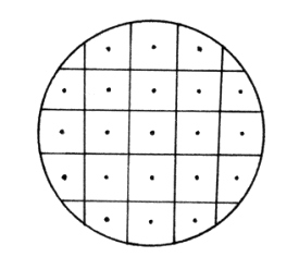
Figure 5.1. The detector surface divided into several sampling areas. The dotted points are the initial points of the trajectory.

5.1.2 Determination of the solid angle

For a given energy, starting from a particular point on the detector and with a particular set of polar and azimuthal angles, the motion of this particle is observed inside the sensor subsystem. The coordinates of these points are included in Appendix D. The equations of motion:

dX/dt = V

M dV/dt = q/c V � B

are solved by Hamming's modified double precision Predictor-Corrector method in a "time reversed sense." "Time reversed sense" because the starting point on the detector surface in this calculation is the end-point of the real particle. At every stage of the trajectory calculation the fate of the particle is determined as discussed later. If this particle's trajectory passes through the open aperture of the sensor subsystem then it is considered as escaped. The polar and the azimuthal angles at the aperture are computed and npas is incremented by one. However, if the particle hits any of the surfaces of the sensor subsystem then it is considered lost and thus ignored since the real particle would also not be able to hit this point on the detector. Then a new set of polar and azimuthal angles is chosen and this process is repeated. Thus, polar and azimuthal are scanned at specific intervals to determine whether the particle escapes or not. A specific range of these for which the particles escape the sensor subsystem forms the set of trajectories that connect the sampling area and the open aperture. Then the solid angle spanned by this set of trajectories is computed using the above equation.

5.1.3 Determination of the fate of the particle

Given the line-segment formed by the points (x_i,y_i,z_i) and (x_i+1,y_i+1,z_i+1) of the trajectory to determine whether the particle is lost or not, the process is as follows:

1. Knowing the coordinates of each of the vertices of the plane polygon, the equations of the planes for all the modelled polygons that comprise the sensor subsystem are determined.
2. Given the line-segment of the trajectory, find whether the line formed by these two points is parallel to a given plane or not.
3. If the line is not parallel then find the intersection point of this line and the plane.
4. Find whether this intersection point belongs to the line segment bounded by (x_i,y_i,z_i) and (x_i+1,y_i+1,z_i+1) or not. If it does not belong to the line segment then the particle has not reached the plane yet and so it is not lost.
5. However, if the intersection point belongs to the line-segment, then determine whether this point lies on the surface of the polygon (finite region of the plane) or not. For all surfaces, except the apertures of the housings of the detectors, deflection system and the opening aperture of the aperture cone, if the particle lies on the surface of the plane polygon then it is considered to be lost, otherwise not. However, if it lies outside the surfaces of the apertures of the housings, deflection system and the aperture cone, it is considered to be lost.

For each of the steps above from (1) to (5) the relevant equations used are included in Appendix C.

In this way, the trajectory calculation continues until a decision is made as to whether the particle hits any of the surfaces and is lost or it passes through the opening aperture and escapes.

5.2 Discussion of the Results

Since at every stage in the particle's trajectory its curvature is determined by the local relation,

r = mcv/Bq    (in c.g.s. units)

the deflection of the low energy electrons should be more than that of the high energy ones. This explains the fact that the Beta detector, which is closer to the opening aperture than Gamma, primarily collects low energy electrons while the Gamma detector collects higher energy electrons.

On examining the trajectories of the particles of different energies emanating either from the Beta detector or the Gamma detector, we do observe that the low energy electrons are indeed deflected more than the high energy ones. This also manifests itself in the shift of the azimuthal angles for which the particles escape, from lower angles to higher angles, as the energy increases. For example, for the energy E=480 keV the range of azimuthal angles for a point on the Gamma detector is 167 to 227 deg. while for the same point for energy E=720 keV the range has shifted to 181 to 228 deg. 

Also, for a particular energy, due to the inhomogeneity of the magnetic field, the curvature of the trajectory of the particle depends upon its position in the deflection system. In this time reversed calculation, the particles entering the deflection system into the region where the field is higher have higher curvatures (less radii) whilst those particles that enter into the region of lower field have lower curvatures (high radii).

Together with this field inhomogeneity which shapes the trajectory of the particles, the surfaces of the sensor subsystem restrict the values of the angles for which the particles escape to a finite range instead of all the allowable values.

Besides, we also expect the symmetry about the z = 0.0 plane in the magnetic field and in the modelled sensor subsystem, to be reflected in the angular distributions of the escaping particles at the detectors and at the apertures.

1. The particles that escape from a point on the z = 0.0 plane of the detector should have an even distribution in the polar angle (theta) about q = 90 deg, i.e. if the particle passes for a polar angle q = 85 deg then there should be corresponding pass for the angle q = 95 deg also. This symmetry about q = 90 deg is well demonstrated by the plots of angular distribution (see figures 5.8 to 5.13) for particles of various energies emanating from the point z = 0.0 of the detectors.
2. Also, the number of particles that escape from the two points situated on either side of z = 0.0 plane of the detector should be the same. This is presented in the plots (see figures 5.14 to 5.16) that show the angular distribution of the escaping particles. Although these particles have the same range of the azimuthal angles, the distribution of the polar angles about q = 90 deg is not symmetric. This is because while scanning over q < 90 deg it hits one of the side surfaces sooner or later than the corresponding side for scans q > 90 deg depending upon its position about the z = 0.0 plane.

The above observations support the validity and the correctness of the magnetic field model.

5.2.1 Variation of the geometric factors with energy

Table 5.1. Geometric factors for different energies for the Beta and the Gamma detectors

5.2.2 Tables of the number of particles that pass

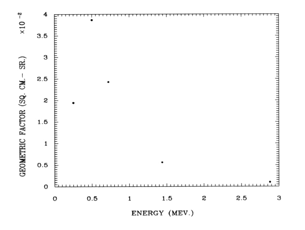
Figure 5.2. Variation of the geometric factors with energy for the Gamma detector.

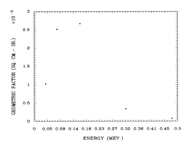
Figure 5.3. Variation of the geometric factors with energy for the Beta detector.

Figure 5.4. Points on the Gamma detector which are the initial points of the trajectories.

Table 5.2. Number of particles that pass for different points on the Gamma detector for E=500 keV. Note: The scanning intervals Dq, Df = 2 deg.

Table 5.3. Number of particles that pass for different points on the Gamma detector for E=720 keV. Note: The scanning intervals Dq, Df = 1 deg for point marked by *, for all others, Dq,Df = 2 deg.

Table 5.4. Number of particles that pass for different points on the Gamma detector for E=1440 keV. Note: The scanning intervals Dq, Df = 2 deg and for points marked *, Dq, Df = 2 deg.

Table 5.5. Number of particles that pass for different points on the Gamma detector for E=2880 keV. Note: The scanning intervals Dq, Df = 1 deg.

Figure 5.5. Points on the Beta detector which are the initial points of the trajectories.

Table 5.6. Number of particles that pass for different points on the Beta detector for E=40 keV. Note: The scanning intervals Dq = 2 deg. For points marked by *, Df = 4 deg, for others Df = 2 deg.

Table 5.7. Number of particles that pass for different points on the Beta detector for E=80 keV. Note: The scanning intervals Dq = 2 deg. For points marked by *, Df = 2 deg, for others Df = 4 deg.

Table 5.8. Number of particles that pass for different points on the Beta detector for E=160 keV. Note: The scanning intervals Dq = 2 deg. and Df = 4 deg.

Table 5.9. Number of particles that pass for different points on the Beta detector for E=320 keV. Note: The scanning intervals Dq,Df = 1 deg.

Table 5.10. Number of particles that pass for different points on the Beta detector for E=480 keV. Note: The scanning intervals Dq,Df = 1 deg.

Additional Figures:

• Figure 5.6. Particle trajectories emanating from the point
  (-0.537177,-0.570312,0.0) of the Gamma detector.
• Figure 5.7. Particle trajectories emanating from the point
  (-0.718812,-0.09375,0.0) of the Beta detector.
• Figure 5.8. Angular distribution for energy E=720 keV.
• Figure 5.9. Angular distribution for energy E=1440 keV.
• Figure 5.10. Angular distribution for energy E=2880 keV.
• Figure 5.11. Angular distribution for energy E=80 keV.
• Figure 5.12. Angular distribution for energy E=320 keV (at the point
  (-0.718812,-0.09375,0.0) and at the aperture).
• Figure 5.13. Angular distribution for energy E=480 keV.
• Figure 5.14. Angular distribution for energy E=320 keV (at the point
  (-0.718812,-0.09375,-0.02384) and at the aperture).
• Figure 5.15. Angular distribution for energy E=320 keV (at the point
  (-0.718812,-0.09375,0.02384) and at the aperture).
• Figure 5.16. Points on the detector Beta which sample the area.

Appendix A
Return to thesis table of contents.

Return to Voyager LECP Data Analysis Handbook Table of Contents.
Return to Fundamental Technologies Home Page.

Last modified 12/9/02, Tizby Hunt-Ward
tizby@ftecs.com